White Wine Quality Exploratory Data Analysis With R 🍷
========================================================
The white wine quality dataset consists of 13 variables, with 4898 observations. Note that the quality was determined by at least three different wine experts. Let us see what makes the best white wine! First we run the summary() function in R and get overwhelmed.
##        X        fixed.acidity    volatile.acidity  citric.acid
##  Min.   :   1   Min.   : 3.800   Min.   :0.0800   Min.   :0.0000
##  1st Qu.:1225   1st Qu.: 6.300   1st Qu.:0.2100   1st Qu.:0.2700
##  Median :2450   Median : 6.800   Median :0.2600   Median :0.3200
##  Mean   :2450   Mean   : 6.855   Mean   :0.2782   Mean   :0.3342
##  3rd Qu.:3674   3rd Qu.: 7.300   3rd Qu.:0.3200   3rd Qu.:0.3900
##  Max.   :4898   Max.   :14.200   Max.   :1.1000   Max.   :1.6600
##  residual.sugar     chlorides       free.sulfur.dioxide total.sulfur.dioxide
##  Min.   : 0.600   Min.   :0.00900   Min.   :  2.00      Min.   :  9.0
##  1st Qu.: 1.700   1st Qu.:0.03600   1st Qu.: 23.00      1st Qu.:108.0
##  Median : 5.200   Median :0.04300   Median : 34.00      Median :134.0
##  Mean   : 6.391   Mean   :0.04577   Mean   : 35.31      Mean   :138.4
##  3rd Qu.: 9.900   3rd Qu.:0.05000   3rd Qu.: 46.00      3rd Qu.:167.0
##  Max.   :65.800   Max.   :0.34600   Max.   :289.00      Max.   :440.0
##     density             pH          sulphates         alcohol
##  Min.   :0.9871   Min.   :2.720   Min.   :0.2200   Min.   : 8.00
##  1st Qu.:0.9917   1st Qu.:3.090   1st Qu.:0.4100   1st Qu.: 9.50
##  Median :0.9937   Median :3.180   Median :0.4700   Median :10.40
##  Mean   :0.9940   Mean   :3.188   Mean   :0.4898   Mean   :10.51
##  3rd Qu.:0.9961   3rd Qu.:3.280   3rd Qu.:0.5500   3rd Qu.:11.40
##  Max.   :1.0390   Max.   :3.820   Max.   :1.0800   Max.   :14.20
##     quality
##  Min.   :3.000
##  1st Qu.:5.000
##  Median :6.000
##  Mean   :5.878
##  3rd Qu.:6.000
##  Max.   :9.000
Fixed.volatile.acidity, citric.acid, fixed.acidity, total.sulfur.dioxide, chlorides, free.sulfur.dioxide, sulphates – I have no idea what there are since I’m not a chemist. The point of this project to explore with data analysis so it is okay. Rest variables are self-explanatory except pH which is how ripe the ingredient used for the wine was. We are most interested in what makes the differences in experts’ wine ratings.
Univariate Plots Section
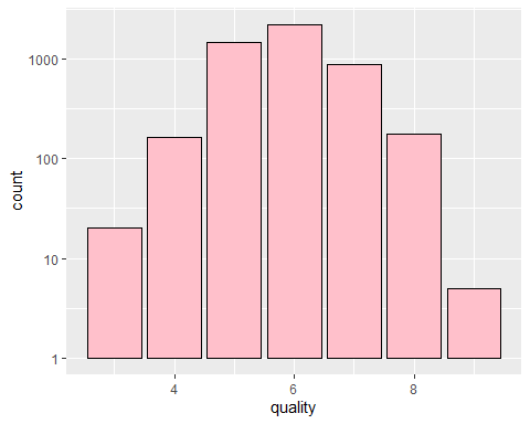
*It looks like Majority of our wines are quality between ‘5’ to ‘7’. There are less than 10 of the highest quality ‘9’ and dataset is normally distributed.
*Let’s look at some boring histograms of rest of the variables.


## `stat_bin()` using `bins = 30`. Pick better value with `binwidth`.

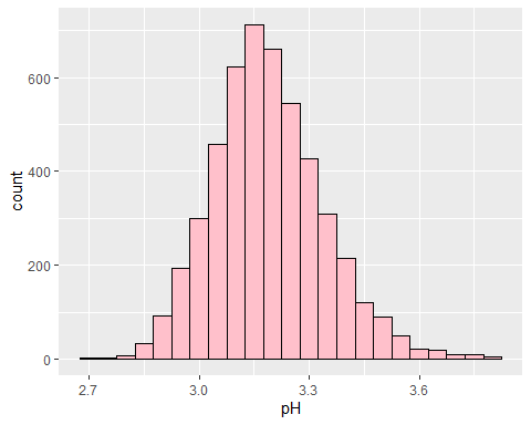

Boring as expected.
Some interesting points:
- Since the dataset consists of real experts (human in the end), I think majority of their points comes from sweetness(sugar), acidity, alcohol and density.
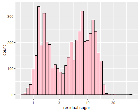
- Sugar had two main peaks at around 2 and 10. I guess majority of winemakers like to make their wine either sweet or not sweet. Most datas were skewed due to very few extreme outliers.
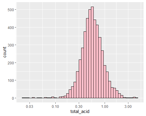
- I have created total_acidity variable which does not make any sense but simplifies fixed, volatile and citric acids and free_rate which is proportion of free sulfur dioxide in total sulfur dioxide. Both for small dimension reduction purpose.
One shot look at all bivariates
## [1] "residual.sugar" "chlorides"      "density"        "pH"
## [5] "sulphates"      "alcohol"        "quality"        "total_acid"
## [9] "free_rate"
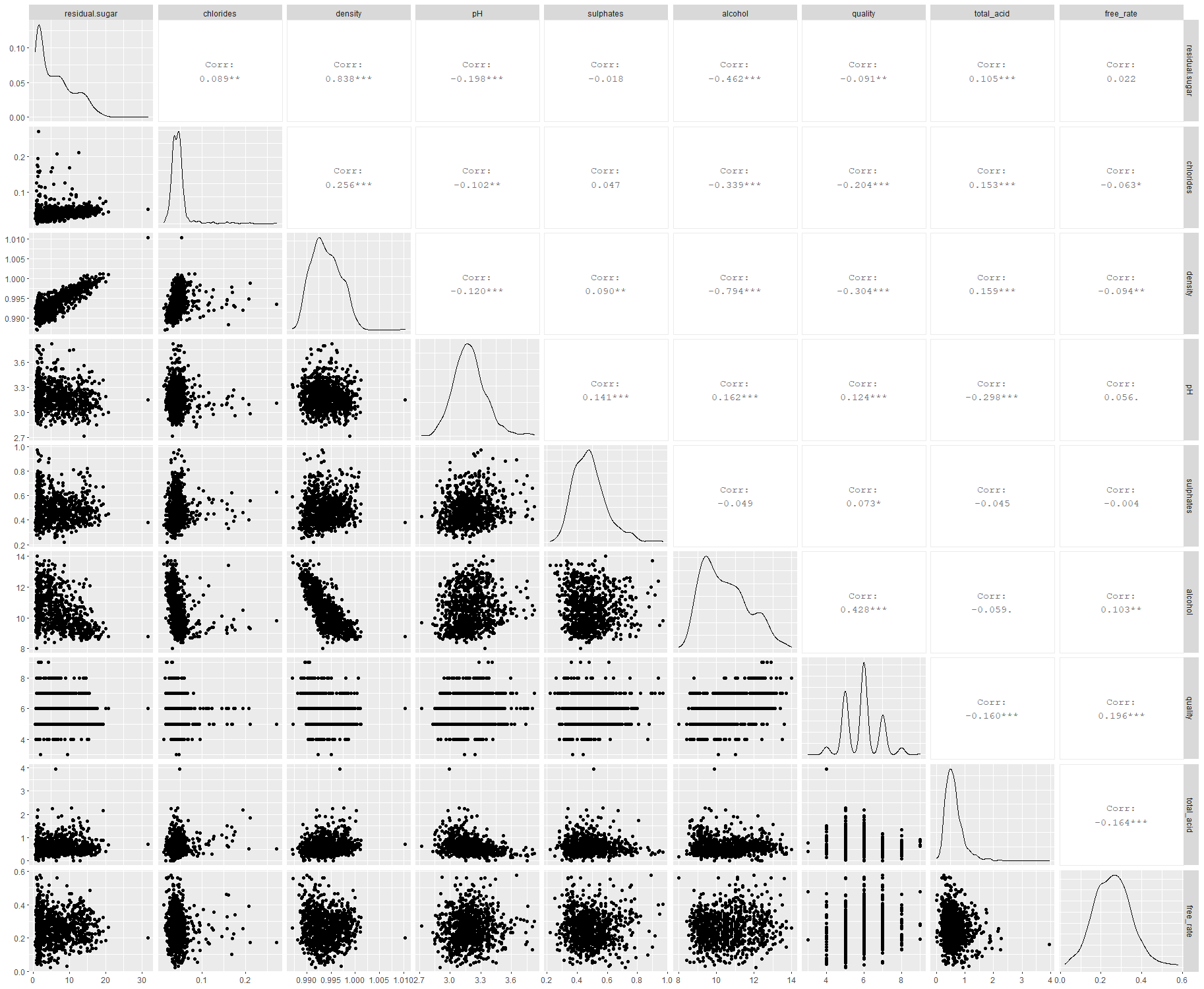
We can see that most scatterplots tends to form clusters with some outliers. Most interesting findings are…
-
Quality is most correlated with alcohol, density, chlorides
-
Alcohol is highly correlated with chloride(-0.82) and sugar(-0.46)
-
Sugar, alcohol and density are highly correlated
Let’s have a closer look.
## [1] "(2,4]" "(4,7]" "(7,9]"
# 3,4 are “Low”, 5,6,7 are “Medium” 8,9 are “High”
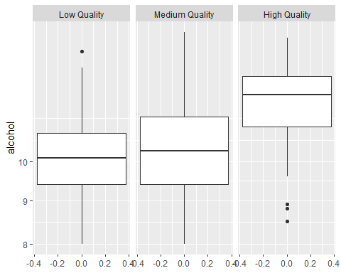
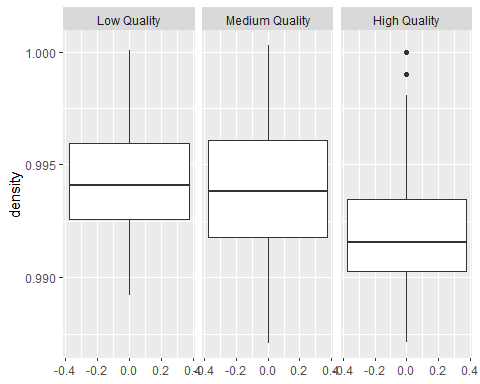

Boxplots of different qualities
So clearly, high quality wines tend to have higher alcohol, lower density and lower chlorides than other qualities of wine.
## `summarise()` ungrouping output (override with `.groups` argument)
## # A tibble: 7 x 5
##   quality med_alcohol med_desity med_chloride     n
##     <int>       <dbl>      <dbl>        <dbl> <int>
## 1       3        10.4      0.994        0.041    20
## 2       4        10.1      0.994        0.046   163
## 3       5         9.5      0.995        0.047  1457
## 4       6        10.5      0.994        0.043  2198
## 5       7        11.4      0.992        0.037   880
## 6       8        12        0.992        0.036   175
## 7       9        12.5      0.990        0.031     5
We used median here since most variables were severly skewed. We can somewhat guess typical characteristics of particular qualities in this chart. We can also see clear difference between quality 3 and 9 instantly.
Multivariate Plots Section
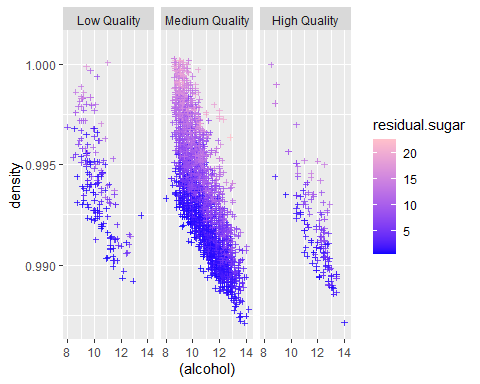
Multivariate Section
There’s a lot going on here. First we can easily confirm that indeed density, alcohol and sugar closely related.
1. Higher sugar levels cover upper right region while lower sugar level covers lower left region. This means higher density and alcohol, higher the sugar level and vice versa.
2. Alcohol and density are highly correlated. I suspect this is because alcohol is main source of reducing density since every other ingredients are likely to increase density.
3. High quality wines have a cluster at the higher alcohol and lower density quadrant. In contrast, low quality wines have a cluster located further towards 1st and 3rd quadrants. Medium quality wines covers both area.
4. No wines seem to exist lowest alcohol and lowest density region.
Multivariate Linear Regression
##
## Call:
## lm(formula = quality ~ density + alcohol + chlorides, data = wine)
##
## Residuals:
##     Min      1Q  Median      3Q     Max
## -3.5904 -0.5209 -0.0050  0.4832  3.0653
##
## Coefficients:
##              Estimate Std. Error t value Pr(>|t|)
## (Intercept) -21.15016    6.16220  -3.432 0.000604 ***
## density      23.67087    6.07373   3.897 9.86e-05 ***
## alcohol       0.34312    0.01529  22.439  < 2e-16 ***
## chlorides    -2.38226    0.55760  -4.272 1.97e-05 ***
## ---
## Signif. codes:  0 '***' 0.001 '**' 0.01 '*' 0.05 '.' 0.1 ' ' 1
##
## Residual standard error: 0.7946 on 4894 degrees of freedom
## Multiple R-squared:  0.1955, Adjusted R-squared:  0.195
## F-statistic: 396.3 on 3 and 4894 DF,  p-value: < 2.2e-16
Of course this is just a old textbook solution. It is terrible and very time consuming to try different variable combinations. Lets use random forest instead.
Random Forest Classifier on all quality [3,9]
## randomForest 4.6-14
##
## Call:
##  randomForest(formula = factor(quality) ~ ., data = train, ntree = 500,      importance = TRUE)
##                Type of random forest: classification
##                      Number of trees: 500
## No. of variables tried at each split: 3
##
##         OOB estimate of  error rate: 31.73%
## Confusion matrix:
##   3  4   5    6   7  8 9 class.error
## 3 0  0   6    5   1  0 0   1.0000000
## 4 0 24  57   43   2  0 0   0.8095238
## 5 0  3 757  367  13  1 0   0.3365469
## 6 0  2 216 1440 103  2 0   0.1832104
## 7 0  0  12  314 391  3 0   0.4569444
## 8 0  0   2   45  41 63 0   0.5827815
## 9 0  0   0    2   3  0 0   1.0000000
We got an accuracy of 69.4%. It is probably hard even for experts to distinguish quality level difference of 1 perfectly.
RFC(All quality) Interpretation (MeanDecreaseAccuracy, MeanDecreaseGini)
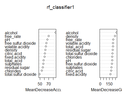
- To explain a little about the plots, MeanDecreaseAccuracy tells us how bad our predictions become if we were to omit that variable completly. MeanDecreaseGini tells us how clean the splits are if that variable was used to split the data.
- This had me wonder if I bucket some quality together into only 3 qualities, ‘High’, ‘Medium’, and ‘Low’ I should be able to increase accuracy by a significant amount.
Random Forest Classifier on bucketed quality (High, Med, Low)
##
## Call:
##  randomForest(formula = factor(quality.bucket) ~ ., data = train,      ntree = 500, importance = TRUE)
##                Type of random forest: classification
##                      Number of trees: 500
## No. of variables tried at each split: 3
##
##         OOB estimate of  error rate: 5.59%
## Confusion matrix:
##            Low Qual. Med. Qual. High Qual. class.error
## Low Qual.         26        112          0 0.811594203
## Med. Qual.        11       3610          3 0.003863135
## High Qual.         0         93         63 0.596153846
Ok we’ve achieved 94.46% accuracy.
RFC(bucketed) Interpretation (MeanDecreaseAccuracy, MeanDecreaseGini)

##             predicted
##              Low Qual. Med. Qual. High Qual.
##   Low Qual.          9         36          0
##   Med. Qual.         7        904          0
##   High Qual.         0         14         10
93.82% accuracy on our test set! So it looks like there barely any overfitting and it generalizes really well too. We can also note that alcohol once again is most important by a significant amount. Followed by many acids and density & sugar giving little meanings.
RFC(bucketed) Interpretation 2 (ROC Curve)
https://www.blopig.com/blog/2017/04/a-very-basic-introduction-to-random-forests-using-r/ (Reference)
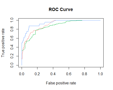
## [[1]]
## [1] 0.8978966
##
## [[1]]
## [1] 0.8655801
##
## [[1]]
## [1] 0.9413354
Red - Low Qual., Green - Med Qual., Blue - High Qual. Here we can see that model is very good at picking out the low quality wines but have harder time picking out high quality wines.In fact, if you recall the 7 level quality model, that model didn’t predict any sample to be high quality. So we can conclude that bad wines are easy to distinguish but best wines are hard to detect.
Reflection
The white wine set contains information on almost 5000 wine data which all have been evaluated by at least 3 different wine experts. We explored many variables and predicted that since density, chlorides, and alcohol had high correlation, their combination will define the quality of any wine. We also looked at an interesting relationship between chemicals like sugar makes density go up and alcohol go down.
Our random forest quantifier agreed with alcohol being important but disagreed with density and chloride being important. Instead it told us a lot of acids which had little to no correlation were very important. And proceeded to succesfully predict 94.46% on training set and 93.82% on test set. Also note it had harder time distinguishing higher quality wines than lower quality wines by looking at its MeanDecreaseAccuracy. Meaning other factors such as presentation or color may may be necessary divide the ‘best wine’ from good wines.
In conclusion, as predicted from my idea; acidity, sweetness, alcohol level but density plays a very important factor in determining high quality white wines. So although I’ve never had wine in my life, I can taste one and tell if it is good or not : )